Guide 2: script management, coding principles and working in the SRS

Scripts needed for this guide

• 00a_run_cleaning.r
• 00b_prelim.r

Introduction

Working with administrative data involves a significant amount of data management and processing before you have an analysis-ready dataset. For novices, this can sometimes be one of the most challenging aspects of working with administrative data. Even experienced researchers may never have received any formal data management training. While the data have undergone various checks and cleaning (for example, on submission to the Department for Education and NHS England), this does not mean they are ready for running analyses. In addition, ECHILD data are held in over 600 tables, some containing hundreds of variables. While most projects will only ever have access to a subset of these, there will still be a very large amount of data to manage and process. Good coding practice is therefore essential to work effectively with the data and minimise disruption when you inevitably find errors or make changes to steps earlier in your processing pipeline.

Data are held on a SQL server

All ECHILD data are stored on a Structured Query Language (SQL) server. Details of the server and database name are confidential and cannot be exported from the Secure Research Service (SRS). You will therefore need to obtain this information from ONS. Documentation should be in your project share.

Because data are stored on a SQL server, you will need to use SQL queries to extract the data. SQL queries are a specialist syntax for working with databases. You only need a very basic knowledge of SQL. In these guides, we show you how to extract data from the SQL server directly into R. To do this, we embed a very simple SQL SELECT query into the R script. A SELECT query has the form as shown in Code Snippet 1, where the asterisk means “all columns.” Square brackets around table and column names are optional. If you ran this query when connected to a database, you would select everything from the table. You could always just do this and carry out further operations in R.

Code Snippet 1 (SQL)

---
SELECT * FROM [table_name]
---

To select just specific columns, you could run a query in the form of Code Snippet 2. Note how each column is separated by a comma. You can put the columns in whatever order you want.

Code Snippet 2 (SQL)

---
SELECT [col1], [col2], [col3] FROM [table_name]
---

In the guides, we usually use a WHERE statement to subset according to certain variables (Code Snippet 3). Here the WHERE statement uses three conditions joined by AND. Note how we explicitly specify [col1] twice in order to select rows where its value lies between two specified values. You could also join by OR and use brackets as you would with any Boolean operation (you will see this in the guides).

Code Snippet 3 (SQL)

---
SELECT * FROM [table_name]
WHERE [col1] >= some_value AND [col1] <= some_other_value AND [col2] = ‘some_string’
---

SQL queries can be more complex than this. If you wish to explore using more advanced queries, a good starting place are the tutorials on W3Schools.

Good memory management

The ONS Secure Research Service (SRS) is a shared resource and the amount of hard disk space allotted to project shares is not infinite. Good memory management is therefore not merely a matter of courtesy to fellow SRS users, but also essential to ensure the smooth running of your projects. In this section of this guide, we offer some easy ways to reduce the amount of information held in memory during a session and, crucially, the amount of space taken up on the hard disk.

More compressed file formats

A major factor to consider is the file format used when writing to hard disk. Table 1 shows the file size of the synthetic data as originally created for the appendix guide, using .csv, R’s .rda format and the .parquet format. It is clear that .csv files are the largest. Indeed, because of this, the ECHILD team actively discourages the use of .csv for saving data. R’s own .rda and .parquet were very similar, with .parquet being slightly smaller when using gzip compression. The .parquet format is “an open source, column-oriented data file format designed for efficient data storage and retrieval”. You can save and load .parquet files in R using the arrow package.

Table 1 also shows how long it took to write the file to disk (on an ordinary desktop computer, not in the SRS). Clearly the fwrite() function (part of the data.table package) is the fastest, though, again, we discourage its use in ECHILD. The .parquet format was quicker than .rda. In this example, the difference is trivial, though you may see a more noticable difference in real-world projects. However, you will also see that, if you follow a similar way of working to these guides, the time factor is not a major concern as you will not be writing to and reading from the hard disk very often.

Table 1. File size and time to save using different file formats (ordered by file size)

File format	Time to save (seconds)	File size (KB)
.csv (write.csv())	12.52	51,270
.csv (fwrite())	0.08	47,364
.parquet (without gzip compression)	0.20	16,143
.rda	2.21	14,262
.parquet (with gzip compression)	0.98	12,018

It should be borne in mind that the above results are applicable to the synthetic data created for the appendix guide. However, we expect that the pattern will be similar in your projects (and it is certainly the case that .csv should be avoided). We therefore recommend using either .rda or .parquet when working with R in ECHILD, both of which result in similar file sizes. In these guides, to keep things simple, we stick to .rda.

Intermediate datasets

One practice that can consume very significant amounts of hard disk space is saving intermediate datasets to disk. These are datasets that are created at steps along the processing pipeline in order to support creating a final dataset at the end. This is a practice we actively discourage except where it is really necessary, where the intermediate dataset contains only absolutely essential information and where it is saved in a highly compressed format. You will see in the guides we do create a few intermediate datasets, but they are all very small on the disk.

In R, avoiding intermediate datasets is easy as R can hold multiple objects in memory at once. Indeed, we could have written the scripts in a way that did not save any intermediate datasets at all. We chose to save some because it made conceptual sense to do so (at the end of processing a particular type of data, for example). This also would make it easier to identify and fix errors or make other changes to particular steps of the pipeline later on. However, we only saved variables that were absolutely necessary and we used a highly compressed file format (R’s own .rda format).

Because Stata used to only allow users to hold one dataset in memory at once, some users find it necessary to save intermediate datasets to disk far more frequently than in R. However, a feature called frames was added with the release of Stata 16 in 2019. This feature enables users to hold multiple data frames in memory at once. While the How To Guides do not have accompanying Stata scripts, we strongly encourage Stata users of ECHILD to consider using frames. You can find out more information on Stata’s website and we use frames in the example Stata scripts accompanying the ECHILD Phenotype Code List Repository.

No redundant data

Only what is essential should be saved to the hard disk. If there is a variable that can easily be recreated in code, consider whether you need to save the derived variable or if you just need to save the source data and recreate the variable each time.

Consider a date. A date value 2025-04-23 in of itself contains all the information that you could possibly need when working with dates. From the single date variable, you can derive year (calendar, financial, academic), month and day. You may, of course, need to work with these latter variables in analysis, but consider whether you need to save them when you save your dataset to the hard disk. The answer may still be “Yes” because of when you need to derive the variables in your data processing pipeline and because of the time this takes, but it is always worth considering whether you do need to save them as columns in addition to the underlying date.

Similarly, once you have cleaned you data, do you need to keep the source data, especially if you are never going to use it again? Do you need to keep rows of data for people not in your cohort? Dropping redundant data will not only reduce the size of the file on the disk, but also the amount of data held in memory. This will make the data easier to handle.

Archiving

At the end of a particular sub-project, consider compressing all project files to free up space in your overall SRS project share. When doing this, consider whether you need to keep any processed data. If you have written your code well, you will be able to entirely reproduce the processed data from your scripts (if it is not possible to do so, then you have not carried out your project in a reproducible manner). We therefore advise deleting processed data before compressing and archiving project files.

Modular, tidy scripts

You will find that, very quickly, you will have written a lot of code. You will need to come back to this code in the future. We also strongly encourage, in the spirit of open research, that you share your code with others. It is therefore important for your and others’ sakes that your code is clear and managed well.

Keeping things short

Keep your scripts short. As long as you have a clear method for keeping your scripts in order, more and shorter scripts are far easier to read and manage than fewer, longer ones. Table 2 shows the total line length of each of the scripts associated with the How To Guides. You will see that the longest script is only 340 lines long. Granted, in real-world projects, you may have to carry out more operations than these scripts, but you can see that you can easily split up your scripts into shorter, more easily manageable ones.

Table 2. Line length of each script

Script	Line length
00a_run_cleaning.r	40
00b_prelim.r	154
01a_identify_npd_cohort.r	202
01b_identify_hes_cohort.r	269
02_npd_demographic_modals.r	340
03_npd_demographic_year7.r	121
04_npd_demographic_ever.r	172
05_hes_birth_characteristics.r	249
06_chc_diagnoses.r	316
07_enrolment.r	119
08_exclusion.r	69
09_absence.r	320
10_exams.r	43
11_outpatient_data.r	68
12_combine.r	230

Writing functions

One way of keeping scripts short is to use functions. Wherever you find yourself copying and pasting code, changing one element a time, in order to carry essentially the same operation (e.g., calculating a rate disaggregated by sub-group), then you have a prime candidate for writing a function instead. Indeed, anything repetitive is a prime target for automation. Functions are preferable to code copied and pasted over and over because:

• It is more interesting to write. Your motivation as a researcher is important, not only to keep you interested in the research process, but because a lack of motivation and concentration can affect the next two points.
• A function is less prone to error. When you copy and paste code, you must remember to change all the elements that must be changed. It is very easy to forget to change something, or change the wrong thing, or change the right thing in the wrong way. Functions are less prone to this because it is much clearer what you are doing and if you need to change the function itself, you only need to do this once. Of course, functions are not completely free of risk of error. You must always carefully test each line of your function to ensure it is behaving as you want it to.
• It is easier to make changes. Imagine you have 80 lines of code because you had to copy and paste several lines of code performing an operation for a particular sub-group. Now imagine you want to change the operation in some way, to calculate a different summary metric or change the groupings, for example. You must either copy and paste another 80 lines of code and edit what needs editing (which comes with the same risks as above) or alter the original 80 lines of code, which also has the same risks but now you may also lose what you originally wrote. It is infinitely easier to edit or create a new function and just run that new function again.

Keep your scripts tidy

Finally, keep your scripts tidy. Take advantage of the fact that RStudio indents for you and use spaces after commas and operators just as you would when writing prose. Examine Code Snippet 4, the first part of which comes from the appendix guide on data.table. The second half is the same, but messy. All lines would run perfectly fine, but it is plain to see the first is preferable.

Code Snippet 4 (R - data.table.demo.r)

---
# Clean version

# Reshape to long
epistart_vars <- names(dt_datatable)[grepl("epistart", names(dt_datatable))]

dt_datatable_long <-
  melt(
    dt_datatable[, c("tokenpersonid", epistart_vars), with = F],
    id.vars = "tokenpersonid",
    value.name = "date"
  )

dt_datatable_long <- dt_datatable_long[order(tokenpersonid)]

# Reshape (back) to wide
dt_datatable_wide <-
  dcast(
    dt_datatable_long,
    formula = tokenpersonid ~ variable
  )


# Messy version

epistart_vars<-names(dt_datatable )[grepl("epistart" ,names(dt_datatable ))]
dt_datatable_long <-melt(dt_datatable[,c("tokenpersonid",epistart_vars),with=F],id.vars="tokenpersonid",value.name="date")
dt_datatable_long<- dt_datatable_long[order(tokenpersonid)]
# Reshape (back) to wide
dt_datatable_wide <-dcast(dt_datatable_long,formula= tokenpersonid ~variable
  )
---

Initialisation

Now let’s turn to the first script that we need to start building our cohort. Open 00a_run_cleaning.r. The first section of this script (Code Snippet 5) sets the working directory, the R library path (necessary when working in the SRS) and loads necessary libraries. Note that system architecture (file structures and connection strings) is confidential and cannot be exported from the SRS. Consult your documentation to find your connection string.

Code Snippet 5 (R - 00a_run_cleaning.r)

---
# Set-up ------------------------------------------------------------------

setwd("[path_omitted]”)
assign(".lib.loc", c(.libPaths(), "path_omitted"), envir = environment(.libPaths))
library(data.table)
library(RODBC)
---

Working directory

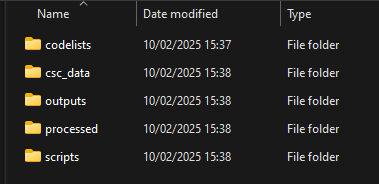
The working directory in all guides assumes a simple structure containing five sub-folders: codelists, csc_data, outputs, processed, scripts (Figure 1). Folder codelists contains phenotype code lists obtained from the ECHILD Phenotype Code List Repository (more information in Guide 7). Folder csc_data contains a copy of the processed CSC data (more information in Guide 12). Folder outputs would contain all outputs from analyses (e.g., tables and graphs, though we never actually use this folder in these guides), processed will contain our processed datasets and scripts contains the R scripts.

Figure 1: An example working directory

R packages

To use R packages in the SRS, the R library path must be set as in Code Snippet 5. We will make use of just two packages: data.table and RODBC. Package data.table makes it significantly easier and quicker to work with data frames, especially large ones, and RODBC enables us to connect to the SQL Server where the data are stored. Consult documentation in your project or contact the SRS helpdesk for help on installing and loading packages if you are having problems.

If you are new to data.table, please read the appendix guide, which provides a brief introduction.

Run scripts

The second part of 00a_run_cleaning.r then runs each of the other scripts in order. The first block creates our basic cohort spine (either from the NPD or HES birth records). The second block carries out data extraction and the third combines the extracted data into our spine.

Each block also runs 00b_prelim.r. This script clears memory, specifies the birth cohorts we are interested in (and the year they will be in year 7) and the ODBC connection string. It also contains a function called mode_fun() and one called clean_hes_data(), to which we will return in subsequent guides.

In 00b_prelim.r, the vector birth_cohorts contains the values 2003 to 2005. In the National Pupil Database, the years (for example, of each census), refer to academic years ending. For example, 2003 refers to the academic year starting in September 2002 and ending in August 2003. We adopt the same convention in these guides, though do keep in mind that the HES is organised according to financial year (April to March) and so in some scripts we make reference to financial years, as well.

You will also see that 00b_prelim.r contains the vector year7_cohorts, which is just birth_cohorts + 12. In other words, in contains the values 2015 to 2017. Again, these will refer to academic years 2014/15 to 2016/17 and are the inception years for our cohort (see Figure 1 of Guide 1).

Coming up…

In the next Guide—Identify a cohort and create a cohort spine—we will run the first substantive script and carry out the actions necessary to create our cohort spine based on a school inception (NPD) cohort or a HES birth records cohort.