Guide 3: identify a cohort and create a cohort spine
Scripts needed for this guide
Introduction
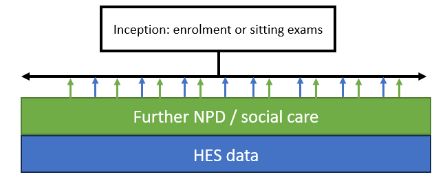
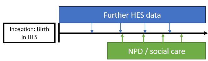
There are two main approaches to defining a cohort in ECHILD: school inception cohorts (Figure 1) and HES cohorts (Figure 2). We will show you a basic approach for both. In either case, further NPD and HES data can be used to ascertain both exposures and outcomes, depending on the purpose of the study. There are, of course, many possibilities and refinements that could be made but we expect that most studies would adopt one of these two basic approaches.
Notes on selection and linkage bias
It is important to recall that, whichever approach you adopt, your study may be subject to selection bias due to the fact that not all births are recorded in HES and that not all children are enrolled in the NPD. Each year, around 7% of children are in other settings (e.g., private schools, home schools or not receiving any education) and children may move in and out of the state sector. The rate at which children become unenrolled from the NPD is associated with various factors such as deprivation, social care experience and special educational needs provision.
Additionally, there may be bias induced by linkage error. Not all children in HES link to NPD records and not all children enrolled in the NPD link to HES records. In accordance with the RECORD statement, you should always report linkage rates for your cohort and, where possible, investigate those who and do not link to inform possible biases in your analyses.
Creating an NPD inception cohort
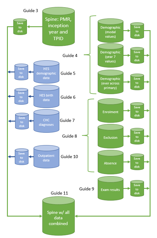
We will start with an NPD inception cohort and move to HES birth cohorts later. When creating a cohort based on the NPD, our general approach to cohort construction is shown in Figure 3. We start by creating a cohort spine that contains Pupil Matching Reference (PMR), inception year and token person ID (TPID). This becomes our master file, onto which we extract and join data later on.
Loading year 7 enrolments
For an NPD inception cohort, we need script 01a_identify_npd_cohort.r. The script starts by identifying children enrolled in year 7 in the autumn, spring and summer censuses of our target academic years (2014/15 to 2016/17). It then also adds in children enrolled in the alternative provision (AP) census, where they are not already included. We would also include the pupil referral unit census had it not been incorporated into the main censuses before our inception years. Finally, we use the NPD-HES bridging file to get the HES TPID.
School censuses
The school censuses present us with two challenges. Each (three terms per year) is stored in its own table on the SQL server and each has different variable names for the same variables. This is because each census has a suffix for each variable name. For example, the column [PupilMatchingRefAnonymous] in the 2015 spring census table (i.e., the spring census for the 2014/15 academic year) is actually called [PupilMatchinfRefAnonymous_SPR15]. That of 2016 is [PupilMatchinfRefAnonymous_SPR16]. A simple for loop that just included [PupilMatchinfRefAnonymous] in a query would therefore not work.
We could write our code that extracts data from each table individually, table by table, query by query, but this will be boring, time-consuming to code, more difficult to change things later (which may lead to errors), inelegant and more difficult to read later. It would be better to loop through the tables and select variables automatically. This is what the first part of our script starts to do (Code Snippet 1).
Code Snippet 1 (R - 01a_identify_npd_cohort.r)
---
dbhandle <- odbcDriverConnect(conn_str)

tables <- subset(sqlTables(dbhandle), TABLE_SCHEM == "dbo")
keep <- tables$TABLE_NAME[grepl("Autumn|Spring|Summer", tables$TABLE_NAME)]
tables <- tables[tables$TABLE_NAME %in% keep, ]

keep <- tables$TABLE_NAME[grepl(paste0(year7_cohorts, collapse = "|"), tables$TABLE_NAME)]
tables <- tables[tables$TABLE_NAME %in% keep, ]

keep <- tables$TABLE_NAME[!grepl("Schools", tables$TABLE_NAME)]
tables <- tables[tables$TABLE_NAME %in% keep, ]

rm(keep)
---
In Code Snippet 1, we first connect to the SQL server using the connection string previously specified and extract the table scheme. This is so we can create a vector (tables$TABLE_NAME) that contains the table names we want. We get all table names on the SQL server, and then only retain those with “Autumn,” “Spring” or “Summer” in their names and then, of these, we retain only those corresponding to our year 7 years. Finally, we remove the tables with “Schools” in their name as these are the school-level censuses, not pupil-level.
Important: When we created these guides, we had access to the data stored in SQL Tables. Non-UCL users of ECHILD will have data provisioned in Views. Views are a pre-calculated version of the original table (in this case the “pre-calculated” version is the whole table). Accessing data in Views is slightly different and, until we update these guides properly, please view this thread on the discussion forum if you are an external user for help in modifying the code so that it works for you.
You will see we use a function called grepl(). This uses regular expressions (a specialist syntax for working with strings) and returns a vector of TRUE and FALSE based on the second argument. In the example in Code Snippet 2, we provide the regular expression "Autumn|Spring|Summer". This means: the string that is “Autumn” or the string that is “Spring” or the string that is “Summer.” In tables$TABLE_NAME are the table names. The function will return a vector of the same length as tables$TABLE_NAME, with a TRUE if any of the three strings are found anywhere in each of the table names, otherwise a FALSE. We then use this to subset the tables$TABLE_NAME vector and store these in the keep object that we use to subset tables.
Code Snippet 2 (R - 01a_identify_npd_cohort.r)
---
keep <- tables$TABLE_NAME[grepl("Autumn|Spring|Summer", tables$TABLE_NAME)]
---
Running up to the end of Code Snippet 1 will give us a data frame (tables) of the tables that correspond to the censuses for year 7 in our cohorts (Code Snippet 3).
Code Snippet 3 (R output)
---
> tables

     TABLE_CAT TABLE_SCHEM         TABLE_NAME TABLE_TYPE REMARKS
377 [OMITTED]         dbo Autumn_Census_2015      TABLE    <NA>
378 [OMITTED]         dbo Autumn_Census_2016      TABLE    <NA>
379 [OMITTED]         dbo Autumn_Census_2017      TABLE    <NA>
658 [OMITTED]         dbo Spring_Census_2015      TABLE    <NA>
659 [OMITTED]         dbo Spring_Census_2016      TABLE    <NA>
660 [OMITTED]         dbo Spring_Census_2017      TABLE    <NA>
691 [OMITTED]         dbo Summer_Census_2015      TABLE    <NA>
692 [OMITTED]         dbo Summer_Census_2016      TABLE    <NA>
693 [OMITTED]         dbo Summer_Census_2017      TABLE    <NA>
---
Next, we create and run a function that loops through these tables and constructs and executes an SQL query (Code Snippet 4) for each, saving the output in an object cohort_spine. This object will be the focal point of all our data management and analyses.
Code Snippet 4 (R - 01a_identify_npd_cohort.r)
---
generate_npd_source <- function() {

  npd_source <- data.table()

  for (table_name in unique(tables$TABLE_NAME)) {

    gc()
    print(paste0("Now doing table: ", table_name))

    temp <-
      sqlQuery(
        dbhandle,
        paste0("SELECT * FROM INFORMATION_SCHEMA.COLUMNS WHERE TABLE_NAME =  '", table_name, "'")
      )

    temp_columns <- temp$COLUMN_NAME
    temp_columns_lower <- tolower(temp_columns)

    pupil_column <- grepl("pupilmatchingrefanonymous", temp_columns_lower)
    age_column <- grepl("^ageatstartofacademicyear", temp_columns_lower)
    ncyearactualcolumn <- grepl("ncyearactual", temp_columns_lower)

    pupil_column <- temp_columns[pupil_column]
    age_column <- temp_columns[age_column]
    ncyearactualcolumn <- temp_columns[ncyearactualcolumn]

    temp <- data.table(
      sqlQuery(
        dbhandle, paste0(
          "SELECT ",
          pupil_column, ", ",
          age_column, ", ",
          ncyearactualcolumn, " FROM ", table_name,
          " WHERE ", ncyearactualcolumn, " = '7' OR ",
          " (", ncyearactualcolumn, " = 'X' AND ", age_column, " = '11')")
        )
      )

    temp[, census := tolower(table_name)]
    temp[, census_year := gsub("[a-z]*_census_", "", census)]
    temp[, census_term := gsub("_census_[0-9].*", "", census)]
    temp[, census := NULL]

    colnames(temp) <-
      c("PupilMatchingRefAnonymous",
        "ageatstartofacademicyear",
        "ncyearactual",
        "census_year",
        "census_term"
      )

    npd_source <- rbind(npd_source, temp)

  }

  npd_source[, census_year := as.integer(census_year)]
  return(npd_source)
}

cohort_spine <- generate_npd_source()
---
At first sight, Code Snippet 4 is a very complex operation, but all that is happening is that we first extract the column names from each table. We have to do this because each table has different names, as described above. We then again use grepl() to find and keep only the names of the columns that we are interested in: [PupilMatchingRefAnonymous], [AgeAtStartOfAcademicYear] and [NCYearActual] (current National Curriculum year). We then just use paste0() to knit these elements together into an SQL query that selects these columns where school year is 7 (you can run each line of the loop independently up to and including the paste0() function to see exactly what the query is that is being created).
Some children do not follow the national curriculum, e.g., those in special schools, and are therefore not in a year. These children have an X for NCYearActual. We include them if they are aged 11 at the start of the year. We then extract some information to create the census year and term columns using the gsub() function (which uses regular expressions to provide a substitute wherever the expression is found), rename the columns and rbind() our query results to the previous steps of the loop.
You may have noticed that the regular expression used to select the age column begins with a circumflex character (Code Snippet 5). In the syntax of regular expressions, this means “only from the beginning.” This is necessary because there is another column, [MonthPartOfAgeAtStartOfAcademicYear]. If we did not include the circumflex, grepl() would have returned a TRUE for the age column we want as well as this one. This would cause an error (try running the code without the circumflex and see what happens).
Code Snippet 5 (R - 01a_identify_npd_cohort.r)
---
age_column <- grepl("^ageatstartofacademicyear", temp_columns_lower)
---
The final bit of the first part of this script then does a few more things (Code Snippet 6). First, we deduplicate based on PMR and census year. In other words, we only want one record per child per birth cohort. However, there is a very small number of children who appear in year 7 in two or more years. This may be linkage error or it may be that children are held back (though this only happens very rarely in England). You may wish to investigate this further. For now, we keep only the first row per child. Finally, in the interests of parsimony, we drop variables that are no longer required.
Code Snippet 6 (R - 01a_identify_npd_cohort.r)
---
cohort_spine <-
  cohort_spine[
    !duplicated(cohort_spine[, c("PupilMatchingRefAnonymous", "census_year")])
  ]

length(unique(cohort_spine$PupilMatchingRefAnonymous)); nrow(cohort_spine)

cohort_spine[, n_record := seq_len(.N), by = PupilMatchingRefAnonymous]
cohort_spine <- cohort_spine[n_record == 1]
length(unique(cohort_spine$PupilMatchingRefAnonymous)); nrow(cohort_spine)

cohort_spine[, census_term := NULL]
cohort_spine[, n_record := NULL]
cohort_spine[, ageatstartofacademicyear := NULL]
cohort_spine[, ncyearactual := NULL]
---
Alternative Provision (AP)
We must now add records for children enrolled in AP. This is much simpler as these is only one table for all years of AP activity. We therefore just write one SQL query. Note also that we drop children from each of these tables who are already in our cohort. In the end, we add a small number of children enrolled in these providers who are not enrolled in the censuses.
You will also see code for the pupil referral unit census, though this has been commented out as the pupil referral unit census merged with the main census before our inception years.
Token Person ID (TPID)
Loading and selecting the HES TPID is also straightforward. The PMR-TPID links are held in a bridging file. We first load this in its entirety. However, before merging, we drop everyone not in our cohort and then we check to ensure that the number of rows is equal to the number of unique PMRs (Code Snippet 7). If these numbers differed, then we would have duplication which would need to be dealt with first.
Code Snippet 7 (R - 01a_identify_npd_cohort.r)
---
linkage_spine <- linkage_spine[PupilMatchingRefAnonymous %in% cohort_spine$PupilMatchingRefAnonymous]
length(unique(linkage_spine$PupilMatchingRefAnonymous)); nrow(linkage_spine)
---
You will also see how throughout we remove objects using rm() once they have served their purpose.
The result
At the end of this script, you will end up with a data table called cohort_spine that contains the PMR (our primary identifier), the census year that they were enrolled in year 7 and, if available, their TPID. We finally write this object to disk.
Creating a HES birth cohort
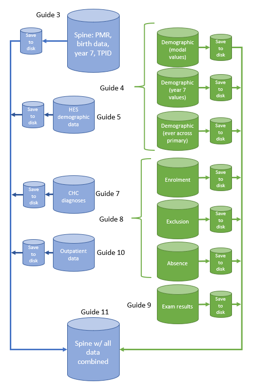
We now turn to the script that creates a HES birth cohort, rather than a school inception cohort: 01b_identify_hes_cohort.r. The same basic approach when starting with a HES birth cohort is the same as above: we start by creating a spine, then load data onto it (Figure 4). The difference is that before, every child had a PMR but not everyone had a TPID. Now, everyone has a TPID, but not a PMR. After this point, all the scripts are identical as we use the same identifiers to link subsequent data (i.e., we use PMR to link data from the NPD and we use TPID to link data from HES). We therefore use the same scripts for all subsequent guides.
We even adopt a very similar approach in extracting the data from HES, whereby we identify relevant tables and loop through them (Code Snippet 8). HES is slightly easier, however, because variables have the same name throughout all years of HES.
Important: When we created these guides, we had access to the data stored in SQL Tables. Non-UCL users of ECHILD will have data provisioned in Views. Views are a pre-calculated version of the original table (in this case the “pre-calculated” version is the whole table). Accessing data in Views is slightly different and, until we update these guides properly, please view this thread on the discussion forum if you are an external user for help in modifying the code so that it works for you.
Code Snippet 8 (R - 01b_identify_hes_cohort.r)
---
extract_hes_data <- function(years) {

  tables <- subset(sqlTables(dbhandle), TABLE_SCHEM == "dbo")

  keep <- tables$TABLE_NAME[grepl("APC", tables$TABLE_NAME)]
  tables <- tables[tables$TABLE_NAME %in% keep, ]

  keep <- tables$TABLE_NAME[grepl(paste0(years, collapse = "|"), tables$TABLE_NAME)]
  tables <- tables[tables$TABLE_NAME %in% keep, ]

  hes_source <- data.table()

  for (table_name in unique(tables$TABLE_NAME)) {

    gc()
    print(paste0("Now doing table: ", table_name))

    temp <- data.table(
      sqlQuery(
        dbhandle, paste0(
          "SELECT TOKEN_PERSON_ID, MYDOB, EPISTART, EPIEND, ",
          "ADMIDATE, DISDATE, ADMIMETH, STARTAGE, ",
          "EPITYPE, CLASSPAT, NEOCARE, HRGNHS, ",
          "NUMBABY, DISMETH, EPIKEY, BIRSTAT_1, MATAGE, ",
          "BIRORDR_1, GESTAT_1, BIRWEIT_1, ",
          paste0("DIAG_", sprintf("%02d", 1:20), collapse = ", "), ", ",
          paste0("OPERTN_", sprintf("%02d", 1:24), collapse = ", "),
          " FROM ", table_name)
      )
    )

    temp <- temp[!duplicated(temp)]
    hes_source <- rbind(hes_source, temp)

  }

  setnames(hes_source, colnames(hes_source), tolower(colnames(hes_source)))
  setnames(hes_source, "token_person_id", "tokenpersonid")

  return(hes_source)

}


print("Loading HES data")
birth_records <- extract_hes_data(c(birth_cohorts[1] - 1, birth_cohorts))
birth_records <- birth_records[!duplicated(birth_records)]
birth_records <-
  birth_records[
    epistart >= paste0(min(birth_cohorts) - 1, "-09-01") &
      epistart < paste0(max(birth_cohorts), "-09-01")
]
---
There is, however, one complicating factor: HES is organised in financial years starting, rather than in academic years ending as used in NPD. Therefore, the HES APC file marked 2002 refers to April 2002 to March 2003. Therefore, if we want birth records for children born in academic years 2002/3, 2003/4 and 2004/5 (September 2002 to August 2005), we need to select HES birth years that actually encompass these.
You will therefore see that the years we supply to our custom extract_hes_data() function are not exactly the birth cohort years that we specify in script 00b_prelim.r. In Code Snippet 8, you will see that we supply c(birth_cohorts[1] – 1, birth_cohorts):
birth_cohorts = 2003, 2004, 2005birth_cohorts[1] = 2003birth_cohort[1] – 1 = 2002c(birth_cohorts[1] – 1, birth_cohorts) = 2002, 2003, 2004, 2005
In other words, the vector we supply means our function extracts HES APC records from April 2002 and March 2006. This more than covers the necessary period of September 2002 to August 2005. If we had not added 2002, we would only select HES data from April 2003, too late for our earliest birth cohort, starting September 2002. Additionally, if we did not keep the 2005/6 HES year, we would only select HES data up until March 2005, too early end August 2005.
This is, of course, too much HES data, but in the final line of Code Snippet 8, you can see we then subset the HES data to the actual dates that we need.
Cleaning HES dates
The next bit of the script that differs substantially from the NPD inception version is that we run a function called clean_hes_dates(). This is specified in script 00b_prelim.r (because we use it in more than one script). This is a complex operation that, essentially, first cleans episode and admission start and end dates and then joins temporally contiguous admissions together into single spells.
Working with clean dates is essential in HES, especially if you are interested in factors such as timing of healthcare contacts, duration of hospital admissions and re-admissions. We therefore encourage you to carefully study this function. Run it piece by piece and see what effect it has on the data. The comments should help you understand what each section is doing.
Recall that in HES, each row represents a finished consultant episode. An admission to hospital can consist of one or more episodes. Patients can be transferred between hospitals. These count as separate admissions in HES but often we are interested in a patient’s total spell in hospital. We therefore here join together admissions into spells. Where an admission ends and a new admission begins on the same day, we join them together. Our code also deals with situations where an admission is recorded as ending after a new admission begins.
The rest of the script
The rest of the script is relatively straightforward. The next section identifies birth episodes following the method of Zylbersztejn et al. Next, we carry out some basic cleaning (e.g., removing implausible values), deduplicate the data and derive an academic year of birth variable. We then load the linkage spine (exactly as above) in order to link in the TPID. Finally, we save the dataset!
Summary
In this rather long guide, we have shown you two approaches to creating your cohort spine: one starting with a school inception and one starting with HES birth records. If you are starting with an NPD inception, you will have ended up with a dataset that contains PMR, inception year and, where available, TPID. If you are starting with a HES birth cohort, your dataset will contain TPID, birth characteristics data, academic year of birth and, where available, PMR.
Whichever approach you took, all subsequent scripts are the same. They will use the same IDs to link the relevant data into the spine. The difference, of course, will be one of who is and is not included in your study.
Coming up…
In the next Guide—NPD demographic and SEND data—we will run three scripts that will extract and save demographic data.