Guide 11: combine it all together
Script needed for this guide
Introduction
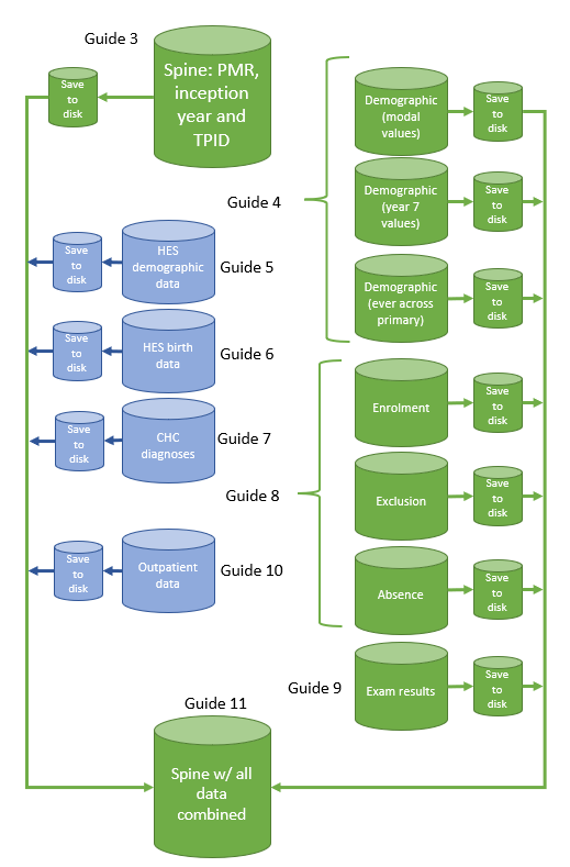
Recall that our plan was to create a master spine, onto which we later join other data (Figure 1, showing the NPD inception scheme). We are now ready to join all the data together in order to produce a single, analysis-ready dataset.
Loading datasets
Script 12_combine.r is perhaps the simplest. However, before we run it, in 00a_run_cleaning.r, we first load all the files that we created up until this point (Code Snippet 1). In Code Snippet 1, note how we create a vector of strings called files, and then remove one file from it. This is the file that we ultimately create at the end of 12_combine.r. You will likely find yourself in a situation where you re-run your scripts and this step just ensures we are combining data into our original spine, not some other (and now incorrect) version of it.
Code Snippet 1 (R - 00a_run_cleaning.r)
---
source("scripts/00b_prelim.r")

files <- list.files("processed/")
files <- files[!(files %in% c("2_cohort_spine_complete.rda"))] # in case it has already been created

for (file in files) { load(paste0("processed/", file)) }
rm(file, files)

source("scripts/12_combine.r")
---
Combining data
We now turn to script 12_combine.r. The basic idea is that we use merge() or we use boolean operators to create flags, depending on the dataset and what kind of variables we need, to combine each dataset with our spine.
NPD demographic data
Starting with the demographics, we merge() the modal demographics file into the spine and create an approximate date of birth variable. NPD only contains month and year of birth but we often need an actual date value and so we arbitrarily create an approximate date of birth on the 15th day of whatever month and year the child was born. We then merge() the year 7 data into the spine. These two merge operations are simple because we only saved one record per child in each of these demographic datasets. Once merged, you should inspect missingness.
The “ever” variables are slightly more complex as the data table we created for them contained a single “ever FSM” variable but yearly SEN data. The general approach, however, is still relatively simple. For FSM, instead of using the merge() function, we exploit the %in% operator to check whether each PMR in the spine exists in the demographics_ever data table where fsm_ever_primary is equal to 1 in that table (Code Snippet 2). This will return, for each child, a TRUE if they ever had FSM in primary school and a FALSE if they did not. Notice how, wherever we use this approach, we subset to rows where the relevant identifier (PMR or TPID) is not missing. This is in order to induce a missing value where the identifier is missing.
Code Snippet 2 (R - 12_combine.r)
---
cohort_spine[!is.na(PupilMatchingRefAnonymous), fsm_ever_primary := PupilMatchingRefAnonymous %in%
               demographics_ever[fsm_ever_primary == 1]$PupilMatchingRefAnonymous]
---
For highest level of SEN, we start by creating a factor variable within our cohort_spine. Then we set its value to the relevant levels, again using the %in% operator in a similar fashion to FSM. We then create a variable that indicates whether the child ever had SEN, meaning we actually have an “ever any SEN” variable as well as a “highest level of SEN” variable (Code Snippet 3).
Code Snippet 3 (R - 12_combine.r)
---
cohort_spine[, highest_sen_primary := factor("None",
                                             levels = c("None",
                                                        "Support",
                                                        "S/EHCP",
                                                        "Specialist provision"))]

cohort_spine[PupilMatchingRefAnonymous %in% demographics_ever[specialist_school == T]$PupilMatchingRefAnonymous,
             highest_sen_primary := "Specialist provision"]

cohort_spine[highest_sen_primary != "Specialist provision" &
               PupilMatchingRefAnonymous %in% demographics_ever[senprovision == "sehcp"]$PupilMatchingRefAnonymous,
             highest_sen_primary := "S/EHCP"]

cohort_spine[highest_sen_primary != "Specialist provision" & highest_sen_primary != "S/EHCP" &
               PupilMatchingRefAnonymous %in% demographics_ever[senprovision == "support"]$PupilMatchingRefAnonymous,
             highest_sen_primary := "Support"]

cohort_spine[, ever_sen_primary := ifelse(highest_sen_primary == "None", F, T)]
---
HES demographics data
Recall that in Guide 5, we provided some hints on how you can adapt our code to extract demographic data from HES. If you did this, remember to also adapt the code here to import it into your spine.
HES birth characteristics
This part is only relevant if you adopted an NPD cohort inception. These are the birth data we extracted in Guide 6. Remember to comment out or delete this section if you do not need it.
Phenotypes
This part deals with the phenotypes. Because you might have multiple phenotypes, we have written a for loop as a way of looping through them all and creating a binary indicator that states whether the child in question ever had a code for each phenotype in question or not (Code Snippet 4). You may want to take a more nuanced approach, for example by only including codes within a certain date range. It is fairly straightforward to amend the code to include a subsetting condition along these lines.
Code Snippet 4 (R - 12_combine.r)
---
for (chc in phen_groups) {

  new_col <- paste0("chc_", chc)
  print(paste0("Now doing ", new_col))

  cohort_spine[, ((new_col)) := as.logical(NA)]
  cohort_spine[, ((new_col)) := tokenpersonid %in% phen_codes[phen_group == chc]$tokenpersonid]

}
---
Non-enrolment, exclusion and absence
The next three sections are quite simple. For non-enrolment, we create binary indicators to show whether the child was NOT enrolled in each of years 8 to 11. We limit to the spring and alternative provision census for the sake of simplicity, but there is no reason why you could not expand this to include other censuses. For exclusion, we simply create a binary variable that indicates the child was excluded in each year. Again, you could separate out fixed-term and permanent exclusions by including an appropriate subsetting condition. The absence data have a few steps. First, we dcast() the data to wide format and then merge() into the spine. For all three outcomes, we also create variables that indicate whether each child ever experienced each of them across secondary school.
Exam data
Given how we extracted the exam data, we get away with a simple merge() here.
Outpatients
With the outpatient data (recall that our dataset contains appointments with pain services), we first create a binary flag indicating “ever” attendance. We then merge the date of the first recorded chronic pain clinic attendance. Remember, as discussed in Guide 10, you may want to consider what to do with cancelled and non-attended appointments, which we ignore here.
Eligibility flag
Before saving, we also create an eligibility flag which declares whether each child was born in the relevant year and linked to HES (i.e., has a TPID) or NPD (i.e., has a PMR), depending on your cohort inception (Code Snippet 3). Strictly speaking, this should probably be in its own script, but we included it here because it was convenient to do so.
Code Snippet 5 (R - 12_combine.r)
---
cohort_spine[, born_in_year := dob_approx >= paste0(min(birth_cohorts) - 1, "-09-01") & dob_approx < paste0(max(birth_cohorts), "-09-01")]
cohort_spine[, eligible := !is.na(tokenpersonid) & born_in_year] # NPD inception cohort
# cohort_spine[, eligible := !is.na(PupilMatchingRefAnonymous) & born_in_year] # HES inception cohort
cohort_spine <- cohort_spine[order(PupilMatchingRefAnonymous, y7_year)]
---
Coming up…
You should now have an analysis-ready dataset. The rest is up to you!
(Though, if you are interested in children’s social care data, you may want to read onto Guide 12 to learn more about that.)